


Tomography 2024, 10(4), 609-617; https://doi.org/10.3390/tomography10040046 - 18 Apr 2024
Abstract
►
Show Figures
Central nervous system tumors produce adverse outcomes in daily life, although low-grade gliomas are rare in adults. In neurological clinics, the state of impairment of executive functions goes unnoticed in the examinations and interviews carried out. For this reason, the objective of this
[...] Read more.
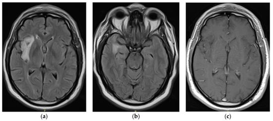
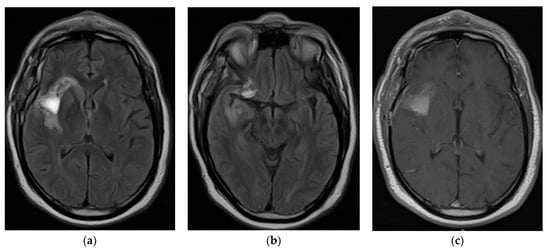
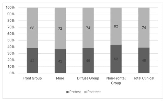
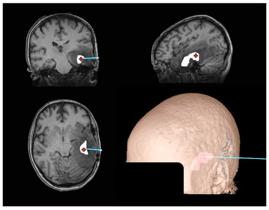
Central nervous system tumors produce adverse outcomes in daily life, although low-grade gliomas are rare in adults. In neurological clinics, the state of impairment of executive functions goes unnoticed in the examinations and interviews carried out. For this reason, the objective of this study was to describe the executive function of a 59-year-old adult neurocancer patient. This study is novel in integrating and demonstrating biological effects and outcomes in performance evaluated by a neuropsychological instrument and psychological interviews. For this purpose, pre- and post-evaluations were carried out of neurological and neuropsychological functioning through neuroimaging techniques (iRM, spectroscopy, electroencephalography), hospital medical history, psychological interviews, and the Wisconsin Card Classification Test (WCST). There was evidence of deterioration in executive performance, as evidenced by the increase in perseverative scores, failure to maintain one’s attitude, and an inability to learn in relation to clinical samples. This information coincides with the evolution of neuroimaging over time. Our case shows that the presence of the tumor is associated with alterations in executive functions that are not very evident in clinical interviews or are explicit in neuropsychological evaluations. In this study, we quantified the degree of impairment of executive functions in a patient with low-grade glioma in a middle-income country where research is scarce.
Full article
Figure 1


